Mushrooms are fun (but deadly)
Published:
In this blogpost I use a popular Kaggle dataset to build class predictive models. The aim is to determine if a mushroom is poisonous or edible based on a minimum number of traits.
Setting the scene
Picture this: it’s been raining all week and you finally get the perfect weekend to go mushroom foraging. Your mushrooming skills aren’t great, but you really want some fresh mushrooms to make a decadent mushroom risotto. The trouble is, will you pick the right mushrooms?

Let’s try and train a model to pick the poisonous mushrooms out for us. We don’t trust our mushroom judgement. We can work with this dataset from Kaggle [1], describing 23 mushroom species from the Lepiota and Agaricus families.
What does the data look like?
Let’s first import some python libraries that will be useful in investigating and manipulating the data:
# Cleaning and exploring data
import pandas as pd
import seaborn as sns
import matplotlib.pyplot as plt
Our dataset is labelled, meaning that we know if the recorded mushrooms are poisonous or edible. Here’s a sneak peak of the data:
| class | cap-shape | cap-surface | cap-color | bruises | odor | gill-attachment | gill-spacing | gill-size | gill-color | stalk-shape | stalk-root | stalk-surface-above-ring | stalk-surface-below-ring | stalk-color-above-ring | stalk-color-below-ring | veil-type | veil-color | ring-number | ring-type | spore-print-color | population | habitat | |
|---|---|---|---|---|---|---|---|---|---|---|---|---|---|---|---|---|---|---|---|---|---|---|---|
| 0 | p | x | s | n | t | p | f | c | n | k | e | e | s | s | w | w | p | w | o | p | k | s | u |
| 1 | e | x | s | y | t | a | f | c | b | k | e | c | s | s | w | w | p | w | o | p | n | n | g |
| 2 | e | b | s | w | t | l | f | c | b | n | e | c | s | s | w | w | p | w | o | p | n | n | m |
| 3 | p | x | y | w | t | p | f | c | n | n | e | e | s | s | w | w | p | w | o | p | k | s | u |
| 4 | e | x | s | g | f | n | f | w | b | k | t | e | s | s | w | w | p | w | o | e | n | a | g |
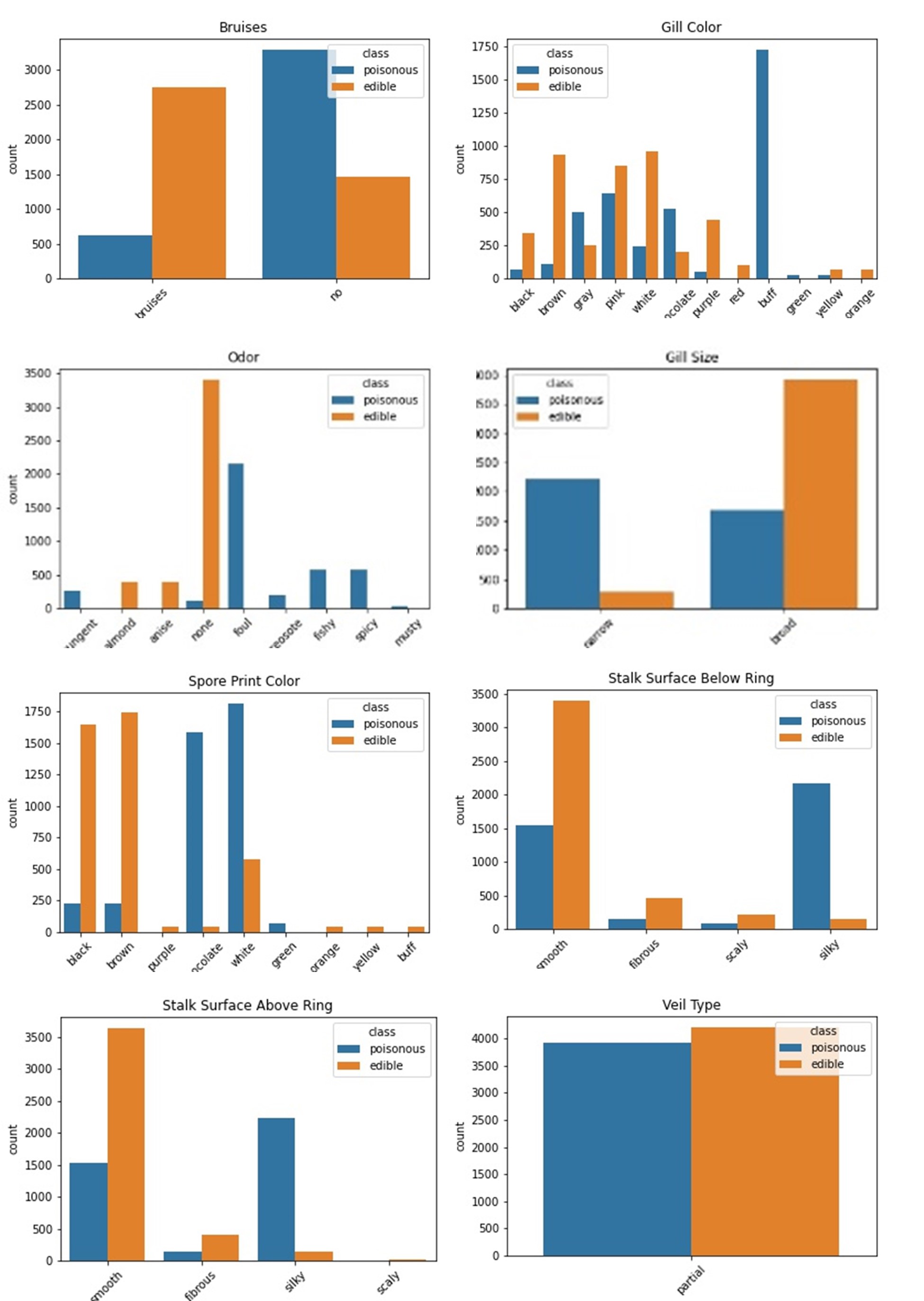
This looks a bit messy. After cleaning up labels by matching them to the data dictionary, we’re able to understand the data better. For example, the first column is ‘class’ with labels ‘p’ and ‘e’ standing for ‘poisonous’ and ‘edible’ respectively, as seen in the data dictionary on Kaggle. Matching these labels with their value in the dictionary for every feature helps us with exploring the data visually. Let’s create some plots to look at each mushroom trait by class:

These are only some of the plots we can create, but they tell us a few important things:
- There’s only one ‘viel_type’ and it is distributed equally between classes; it’s a column that can be dropped.
- There seems to be a big difference in the amount of bruising between poisonous and non-poisonous mushrooms.
- ‘odor’ could be a reliable predictor of mushroom class, as it shows edible and poisonous mushrooms tend to have different smells.
- ‘gill_size’ is generally broader in edible mushrooms and narrower in poisonous.
- A buff ‘gill_colour’ could be a good indicator of a poisonous mushroom.
- Surface above and below stalk might be able to be differentiated between mushroom classes.
- ‘spore_print_colour’ is quite differentiated between classes.
One peculiarity about this data is that for the ‘stalk_root’ trait, one of the possible labels is: ‘missing’. This is probably because it was not recorded for that mushroom, or because there was no stalk root present on the studied sample. We can impute these values with K-Nearest Neighbour clustering (look at my github repo for an example with this data).
Lets summarise the quality of our data so far:
| Feature | dtypes | Count | NAs | Uniques | |
|---|---|---|---|---|---|
| 0 | class | object | 8124 | 0 | [‘poisonous’ ‘edible’] |
| 1 | cap_shape | object | 8124 | 0 | [‘convex’ ‘bell’ ‘sunken’ ‘flat’ ‘knobbed’ ‘conical’] |
| 2 | cap_surface | object | 8124 | 0 | [‘smooth’ ‘scaly’ ‘fibrous’ ‘grooves’] |
| 3 | cap_color | object | 8124 | 0 | [‘brown’ ‘yellow’ ‘white’ ‘gray’ ‘red’ ‘pink’ ‘buff’ ‘purple’ ‘cinnamon’ ‘green’] |
| 4 | bruises | object | 8124 | 0 | [‘bruises’ ‘no’] |
| 5 | odor | object | 8124 | 0 | [‘pungent’ ‘almond’ ‘anise’ ‘none’ ‘foul’ ‘creosote’ ‘fishy’ ‘spicy’ ‘musty’] |
| 6 | gill_attachment | object | 8124 | 0 | [‘free’ ‘attached’] |
| 7 | gill_spacing | object | 8124 | 0 | [‘close’ ‘crowded’] |
| 8 | gill_size | object | 8124 | 0 | [‘narrow’ ‘broad’] |
| 9 | gill_color | object | 8124 | 0 | [‘black’ ‘brown’ ‘gray’ ‘pink’ ‘white’ ‘chocolate’ ‘purple’ ‘red’ ‘buff’ ‘green’ ‘yellow’ ‘orange’] |
| 10 | stalk_shape | object | 8124 | 0 | [‘enlarging’ ‘tapering’] |
| 11 | stalk_root | object | 5644 | 2480 | [‘equal’ ‘club’ ‘bulbous’ ‘rooted’ nan] |
| 12 | stalk_surface_above_ring | object | 8124 | 0 | [‘smooth’ ‘fibrous’ ‘silky’ ‘scaly’] |
| 13 | stalk_surface_below_ring | object | 8124 | 0 | [‘smooth’ ‘fibrous’ ‘scaly’ ‘silky’] |
| 14 | stalk_color_above_ring | object | 8124 | 0 | [‘white’ ‘gray’ ‘pink’ ‘brown’ ‘buff’ ‘red’ ‘orange’ ‘cinnamon’ ‘yellow’] |
| 15 | stalk_color_below_ring | object | 8124 | 0 | [‘white’ ‘pink’ ‘gray’ ‘buff’ ‘brown’ ‘red’ ‘yellow’ ‘orange’ ‘cinnamon’] |
| 16 | veil_type | object | 8124 | 0 | [‘partial’] |
| 17 | veil_color | object | 8124 | 0 | [‘white’ ‘brown’ ‘orange’ ‘yellow’] |
| 18 | ring_number | object | 8124 | 0 | [‘one’ ‘two’ ‘none’] |
| 19 | ring_type | object | 8124 | 0 | [‘pendant’ ‘evanescent’ ‘large’ ‘flaring’ ‘none’] |
| 20 | spore_print_color | object | 8124 | 0 | [‘black’ ‘brown’ ‘purple’ ‘chocolate’ ‘white’ ‘green’ ‘orange’ ‘yellow’ ‘buff’] |
| 21 | population | object | 8124 | 0 | [‘scattered’ ‘numerous’ ‘abundant’ ‘several’ ‘solitary’ ‘clustered’] |
| 22 | habitat | object | 8124 | 0 | [‘urban’ ‘grasses’ ‘meadows’ ‘woods’ ‘paths’ ‘waste’ ‘leaves’] |
Our data looks very clean now, it may be time for some modelling!
Let’s get down to business
So far, we have only needed pandas, matplotlib.pyplot and seaborn to clean and visualise our data. Now that we’re moving on to feature engineering and modelling, let’s define some more imports:
# Modelling
from sklearn.model_selection import train_test_split
from sklearn.tree import DecisionTreeClassifier
from sklearn.linear_model import LogisticRegression

# Evaluating models
from sklearn.metrics import classification_report, confusion_matrix, roc_auc_score, roc_curve
from sklearn import tree
Let’s see what our features and target variable are:
target = 'class'
features = [feature for feature in list(mushroom_data.columns) if feature not in target]

print(features)
['cap_shape', 'cap_surface', 'cap_color', 'bruises', 'odor', 'gill_attachment', 'gill_spacing', 'gill_size', 'gill_color', 'stalk_shape', 'stalk_root', 'stalk_surface_above_ring', 'stalk_surface_below_ring', 'stalk_color_above_ring', 'stalk_color_below_ring', 'veil_color', 'ring_number', 'ring_type', 'spore_print_color', 'population', 'habitat', 'stalk_imputed']
Those are a lot of features! But it’s okay, python can handle it. We next have to seperate our data (column-wise), into features (X) and target (y). Then we should further divide it (row-wise) so that we can test and train our model. Splitting the data in this way helps us evaluate the ‘goodness’ of our model, it helps us see that it’s actually doing what we want! More on that later.
# Define X and y
X = mushroom_data[features]
y = mushroom_data[target]

# Split the data
X_train, X_test, y_train, y_test = train_test_split(X, y, test_size = 0.35, random_state = 40)
Cool. We now how everything we need to start modelling, except that statistical and machine learning models handle data in a numerical format, not in strings like ours is. To transform our data into numerical there are various options:
sklearn.preprocessing.OrdinalEncoder- establishes an ordinal relationship between labels in a variable and gives them numerical values accordingly.sklearn.preprocessing.LabelEncoder- can assign numbers to category labels in a variable randomly or in alphabetical order.pd.get_dummiesa.k.a. One Hot Encoder - attributes each label in a category its own column, meaning that every observation has two possible values: either that label corresponds to them ($1$) or it doesn’t ($0$). This augments the dimensions of our data considerably, especially if we have columns with high cardinality (many unique labels).
There is no ordinality in our mushroom features, so we don’t want to choose the first option. As for the second, it’s very possible that an ordinal relationship in the data is implied with how the numbers are assigned to labels. To avoid this, the third option is best.
One Hot Encoding (OHE) could create errors in some models if we aren’t careful. Especially in parametric machine learning, you want to avoid features being correlated with one another. If we work through an example it will be easier to understand why. The mushroom trait ‘gill_size’ has two possible categories: ‘broad’ or ‘narrow’. Suppose we had 5 observations of mushrooms with two possible gill sizes. OHE this feature would mean we have two new columns, one for each of the types of gill size:
| Observation | gill_size | gill_size_broad | gill_size_narrow |
|---|---|---|---|
| 1 | broad | 1 | 0 |
| 2 | broad | 1 | 0 |
| 3 | narrow | 0 | 1 |
| 4 | broad | 1 | 0 |
| 5 | narrow | 0 | 1 |
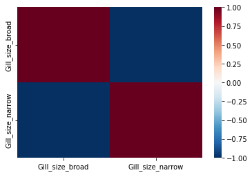
One of the OHE columns can say exactly the same thing as the other, only the numbers for the numeric labels are reversed. This means the columns are dependent of each other, and they could be very correlated. We want features in our model to not be multicollinear, but we do want them to correlate with our target variable. In this case, both of these OHE features correlate perfectly with each other (see the heatmap below), which means we must drop one.

Dropping one of the columns created for each feature is standard practice for all features when we do any OHE, except for when the model in question are works with Euclidean space. That gets a bit more tricky, but we can talk about that another day.
OHE features on python is a breeze, even if we have so many variables, it’s a simple line of code for each data frame:
# Do this for X_train and X_test
X_train_eng = pd.get_dummies(X_train, columns = features, drop_first = True)

# Do this for y_train and y_test
y_train_eng = y_train.map({'edible':0, 'poisonous':1})
The last argument in the get_dummies function is what helps us eliminate one column for every feature. This is not a very mechanistic way of improving our model, nor is it best practice, but it will work for now. .map will do the same binary transformation for our target variable. With our data now in numerical format, we can start modelling!
To choose or not to choose a model
Traditionally, mushrooms are identified using mushroom identification guides (actually it’s just an obsessive amount of practice, but you have to start somewhere). These guides are much like decision trees, where a question is asked about a mushroom trait, which then takes us down a new line of questioning to identify the type of mushroom, and thus, if it’s poisonous. Because of this, I think the most fitting algorithm to run first would be a tree-based one. Let’s start with running a decision tree. From there we can determine which features contribute the most in the model’s decision making power.
# Declare and fit the DecisionTree
dt = DecisionTreeClassifier(random_state = 42)
dt.fit(X_train_eng, y_train_eng)
From here we can test our model’s performance on both the training data and the test data. Lets see how we did:
###################### TRAIN SET ######################

               precision    recall  f1-score   support

           0       1.00      1.00      1.00      2738
           1       1.00      1.00      1.00      2542

    accuracy                           1.00      5280
   macro avg       1.00      1.00      1.00      5280
weighted avg       1.00      1.00      1.00      5280


###################### TEST SET ######################

               precision    recall  f1-score   support

           0       1.00      1.00      1.00      1470
           1       1.00      1.00      1.00      1374

    accuracy                           1.00      2844
   macro avg       1.00      1.00      1.00      2844
weighted avg       1.00      1.00      1.00      2844
Um… It seems we have perfect scores! I am especially interested in maximising recall because it will minimise false negatives (FN - check the confusion matrix below). In other words, we want to minimise the possibility of eating a mushroom based on the prediction that it’s edible when it’s actually posionous… things could go very wrong.
| CONFUSION MATRIX | ||
|---|---|---|
| Actually Poisonous | Actually Edible | |
| Predicted Poisonous | TP | FP |
| Predicted Edible | FN | TN |
From the evaluation metrics printed above, we know that this decision tree is reliable (completely 100% for some bizarre reason that we have absolutely identified). Let’s have a look at what features are most useful in accurately predicting poisonous mushrooms in our feat_imp table (code to extract this from a DecisionTree in my github repo for this project):
| Feature | Gini_Importance | Summed_Importance | |
|---|---|---|---|
| 0 | odor_none | 0.613 | 0.613 |
| 1 | bruises_no | 0.18 | 0.793 |
| 2 | stalk_root_club | 0.065 | 0.858 |
| 3 | stalk_root_rooted | 0.051 | 0.909 |
| 4 | habitat_woods | 0.038 | 0.948 |
| 5 | spore_print_color_green | 0.033 | 0.981 |
| 6 | stalk_color_below_ring_yellow | 0.012 | 0.993 |
| 7 | cap_color_yellow | 0.002 | 0.995 |
| 8 | stalk_surface_above_ring_scaly | 0.002 | 0.997 |
| 9 | cap_surface_grooves | 0.002 | 0.999 |
| 10 | population_clustered | 0.001 | 0.999 |
| 11 | stalk_surface_below_ring_scaly | 0.001 | 1.0 |
| 12 | gill_size_narrow | 0.0 | 1.0 |
| 13 | stalk_color_below_ring_cinnamon | 0.0 | 1.0 |
| 14 | ring_number_two | 0.0 | 1.0 |
The importances are calculated from the DecisionTree using a metric called Gini Impurity, which returns a normalised probability of misclassification for each variable (see documentation here [2]). Unsurprisingly, a lack of odour is a useful feature in the model (the most useful), and it holds over 60% of the predictve power in identifying poisonous mushrooms. We also see a few of the other features we thought would be interesting, which means our EDA was very productive.
Let’s make a new tree with only the top 12 most important features, since they represent almost 100% of the predictive power of the model. A model that is still good with less features is more valuable than one with many features. It’s always good to remember the KISS rule (Keep it Simple, Stupid).
# Select features of interest in training and test sets
select_interesting = list(feat_imp['Feature'][:12])
X_train_important = X_train_eng[select_interesting]
X_test_important = X_test_eng[select_interesting]

# Declare and fit the Decision Tree
dt_important = DecisionTreeClassifier(random_state = 42)
dt_important.fit(X_train_important, y_train_eng)
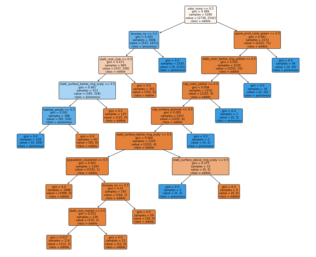
I won’t show you explicitly here again, but we get the exact same perfect evaluation scores as our last model (with less features!). This is great, we can even see what the decisions in the tree look like:

This means using this decision tree will tell us if a mushroom is poisonous after asking at most 9 questions about the mushroom traits, thats pretty good!
Let’s think about good practice
For the sake of being thorough, I was having a look at the practicality of having over 100 OHE features for training, like we do in our first model, specifically for tree-based algorithms. OHE categorical features used in training decision trees is thought to be unwise (for discussions on using sparse data for modelling, see: [3] [4]), so lets have a look at the evaluation output of a logistic regression on the same features, for peace of mind.
###################### TRAIN SET ######################

               precision    recall  f1-score   support

           0       0.99      0.99      0.99      2738
           1       0.99      0.99      0.99      2542

    accuracy                           0.99      5280
   macro avg       0.99      0.99      0.99      5280
weighted avg       0.99      0.99      0.99      5280


###################### TEST SET ######################

               precision    recall  f1-score   support

           0       0.99      0.99      0.99      1470
           1       0.99      0.99      0.99      1374

    accuracy                           0.99      2844
   macro avg       0.99      0.99      0.99      2844
weighted avg       0.99      0.99      0.99      2844
Hmm… There’s no difference between our test and train evaluation scores for this model either, which means our model is performing well, but the scores aren’t as perfect as in our decision tree. Even the littlest bit of error in our recall could be fatal, implying the model is misclassifying poisonous mushrooms.
It’s still surprising that a logistic regression performed worse than a decision tree for this data, when we know that’s the type of linear modelling OHE was devised for! I would personally use the decision tree built from the most important features if you’re out mushroom picking (or mushrooming, as the cool kids say), especially if you’re unsure about your foraging skills!
